Voxelspace in a Compute Shader - Writeup WIP
Introduction
I found out about this algorithm a while back, and have really wanted to do an implementation of for quite some time. I recently got to talking with the GPVM group about it, and got motivated to try to do it in a compute shader.
A couple weeks later, I had something working, and presented at the GPVM meeting. This is the third talk I have given about one of my projects to this group. The subject matter attracted some new attendees, including Wolfgang Engel. You can see the video below, and the slides from this video are available here. The page following expands on the topics covered in the slides and presentation a bit.
Note that the animations below mostly come from this page, written by Sebastian Macke. It has a very comprehensive explanation of the nuts and bolts of this algorithm, including an implementation in a very short snippet of python.
Background
In the earlier days of realtime computer graphics on commodity PCs, people had yet to embrace triangles as the de facto standard method - the hardware then was of orders of magnitude lesser capability than it is today. There were a number of different methods to produce an image, and this "ray surfing" approach is one of them. It's easy to have standards colored by the fidelity of modern approaches, but this really was years ahead of its time. Below, you can see the comparison between two helicopter games, Gunship 2000 ( MicroProse, 1991 ) on the left, and Comanche ( NovaLogic, 1992 ) on the right. The difference in the level of detail between the two is significant. The Comanche example is particularly impressive, considering its release being in the days long before the massive parallel processing capability available in modern GPUs.
The polygon raster budgets of the time were very small by today's standard, only allowing maybe a few hundred triangles to be rendered while keeping interactive framerates. Surprisingly, perhaps, by modern standards, the original implementation of the voxelspace algorithm was computed entirely on the CPU.
Today, when you hear the term 'voxel', you associate it with games like Minecraft, or the innumerable clones thereof. They make no use of voxels in their rendering technology, instead rendering everything purely as mesh data, but that is a topic for another day. In the zeitgeist, the term 'voxel' is inextricably linked with this idea of little cubes. But when you consider the constituent parts of the term, 'volume element', in the same sense that a pixel is a 'picture element', there is no dimensionality encoded in the term. For some more discussion of this topic, consider taking a look through this paper. This voxelspace algorithm was considered a voxel rendering method, in the language of the day. The landscape rendering employed here completely eschews triangles as a rendering method. Instead of considering cubic voxels, it considers these colored columns, encoded in two parts: a texel in a 2d heightmap and corresponding texel in a colormap. When you go through and understand the rendering process, you see that, in fact, this representation does consider them as objects with volume, as elements of a greater whole.
Data Layout & Representation
This program is actually very simple, there are very few parts involved to get it working. The image is produced in a RGBA render texture, and presented with a screen-covering triangle. The image in the texture is output from the compute shader. The compute shader is invoked with a 1d dispatch, by vertical columns across the X of the image. I will explain why this invocation structure is a good fit in the next section.
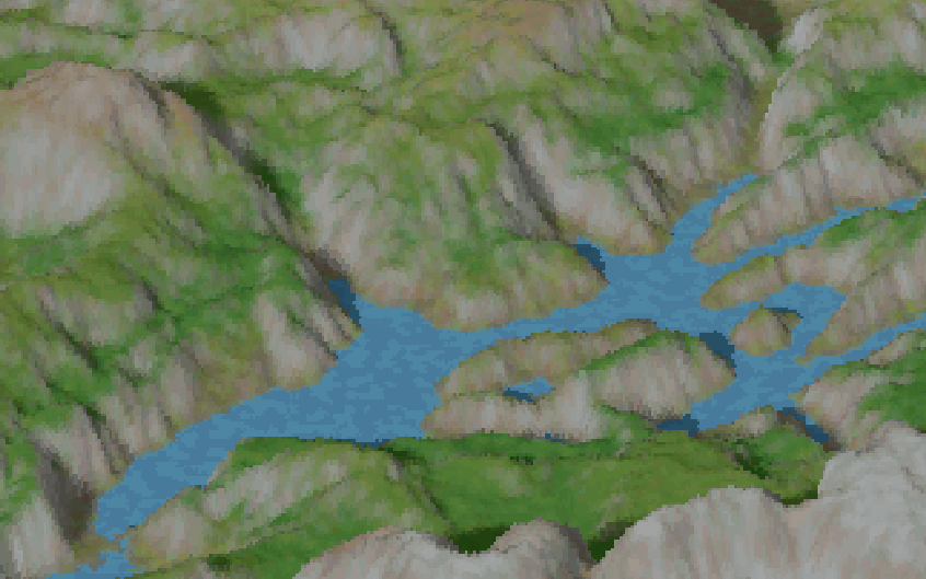
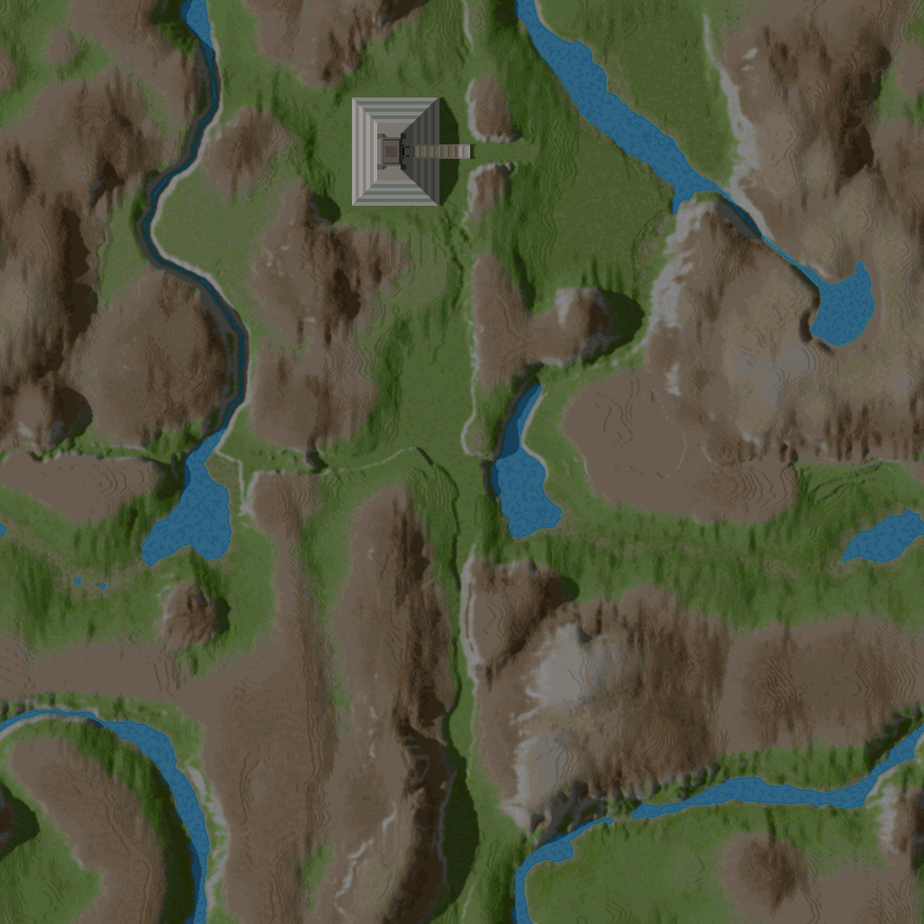
As I mentioned before, the algorithm operates on two pieces of data - the heightmap and the corresponding colormap. You can see an example of what these two textures look light below. The heightmap is a grayscale texture, which encodes the height value of the landscape, at each texel, and the colormap contains the colors. This contains the landscape color as well as baked lighting.
How it Works
Sebastian Macke's resource, mentioned above, describes two ways you might go about this rendering process. I wish to convey the motivation, then the mechanics of how it works. The first method, which we will call the backwards approach, starts at the most distant point and draws towards the viewer. The second, the forwards approach, starts at the viewer and goes out to some maximum distance. The forward approach is an improvement over the backwards approach in pretty much every way you could imagine - it is the result of a very impressive recontextualization of the problem by Kyle Freeman at NovaLogic, and it is a much more efficient solution. I will describe the differences between the two, and why this is the case.
First, what is being done by the backwards approach? As you can see here, by starting at the farthest point, and coming backwards ( with respect to the view direction ), there is a lot of pixel data drawn that becomes irrelevant as closer data is drawn over top. This is a phenomenon called overdraw, and here it is a huge source of inefficiency. Watching the process unfold in the animation above, you can imagine how many pixels are drawn, only to be overwritten by subsequent data closer to the viewer. But how can you know ahead of time, how much of that pixel data is relevant? Before drawing the next closest sweep across, how can you know how much will be kept? How do you reduce this overhead of drawing all these invisible pixels?
The answer to all these questions is the forwards approach. This method starts at the viewer position and goes out into the space, traveling forwards along the view direction. For each vertical strip of pixels, a value is maintained - we call it the ybuffer. Initially zero, it keeps the highest value on the screen which has been drawn to. As you get height data, and translate it to a height on the screen, you know that you only have to draw from the ybuffer value, to the computed height - you will never draw pixels at a y position less than the ybuffer value, because you have already seen pixels drawn which are closer to the viewer. This takes advantage of some inherent limitations of using a heightmap this way - because there can be no overhangs or caves, you can know that this maximum encountered y logic will hold.
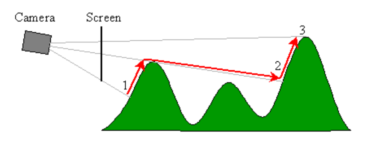
This graphic from the Outcast GDC talk by Appeal illustrates what is going on from another point of view. There's a bit of logic which is well described in Sebastian Macke's writeup, to determine the height on the screen, providing the foreshortening at points further away from the viewer. When you get y values higher on the screen than the previously recorded highest y value, you draw the pixels - otherwise, you skip it and move on to the next height sample. In doing this, you eliminate all the overdraw that takes place in the backwards approach. This view also helps depict the parallelization potential that is afforded by keeping a separate ybuffer value for each vertical strip of pixels - consider this side view as one invocation of a parallel job for every vertical strip. This is where I saw the potential for doing it in a shader - a 1 dimensional dispatch along the x of the image takes advantage of this aspect of the problem.
Changes in View Ray Generation
The original implementation uses two rays that go out into the scene, bounding the image on the left and right. As the rendering process sweeps horizontally across the image, further and further away from the viewer, samples are taken at interpolated positions. This interpolation takes place between points on these two lines, effectively creating a 2d analog to a view frustum.
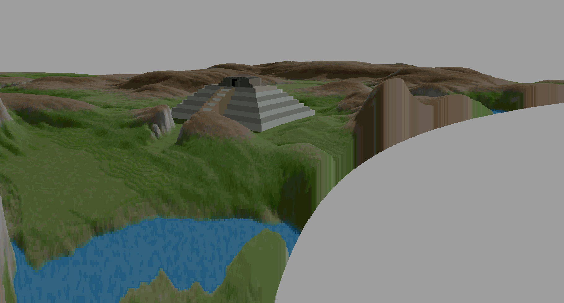
I decided that this was somewhat redundant, as each shader invocation would have to calculate these two points, before interpolating a position at the invocation's X index. I am doubtful that this is in fact very expensive, but I implemented the logic in a different way. Instead of interpolating sample locations, what I did was to map the value [0,x] to the range [-1,1], and use this as a scalar on a variable 'FoV' value, that would rotate the view direction for each shader invocation. If the FoV scalar is turned up too high, you can see behind the viewer, and even have it loop around a few times. You can see what that looks like, in the image below.
Additionally, I implemented a configurable side-to-side offset for the ray origins. This is scaled in the same way the FoV is applied to the rotation, with the base offset defined by the cross product of a vector going straight up with the direction vector. This is used to create more of an orthogonal projection, when the FoV is brought down to a very small value. These offset ray origins can introduce some odd curvature when used in conjuction with a nonzero FoV scalar, as you can see in the image below.
Extending the Basic Implementation
Minimap
I drew inspiration for the minimap from this implementation by Marat Isaw. His implementation, however, is all CPU based, and uses an isometric rendering method, based on the backwards approach described above. The way I did it is to have a smaller dispatch with the same rendering logic, drawing into a second render texture which only covers the upper left corner of the screen. Keeping a transparent background in this render texture, and drawing the resulting image over the main pass render result, you get a little minimap showing a shrunk down view of the area in front of the viewer.
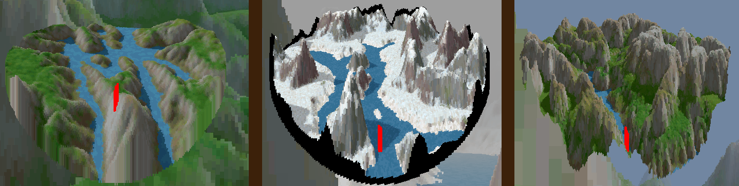
As you can see in this picture, the drawing method is flexible enough to draw the data in a number of very different looking ways. Where a lot of the images on this page depict something more perspective correct, looking like landscape, it's possible to do something more orthogonal. This can be used to show the heightmap content in a way that looks more like a distant view, with little foreshortening. The second pass is done by masking out a small circle on the map, about a position a ways out in front of the viewer's location. This uses a second shader, which hard codes most of the view parameters. The minimap draw shader only takes the view direction and viewer position as uniform inputs.
Shown here, this concept of a minimap went through a couple of iterations. This masked out circle worked well to constrain the view, but it involved a transition from zero height to whatever the heightmap read was when the edge of the masked circle was reached. This manifests as these vertical strips of color. To illustrate the process I went through to fix this, I have expanded the mask very slightly, and replaced the color values with opaque black. This shows the areas in which these vertical strips exist. By replacing the black with full transparency, e.g. alpha equal to zero, I was able to get this appearance of a floating surface. The reason that this works is because of the ybuffered forward approach, where drawing a strip to a certain height precludes any further drawing below that height value.
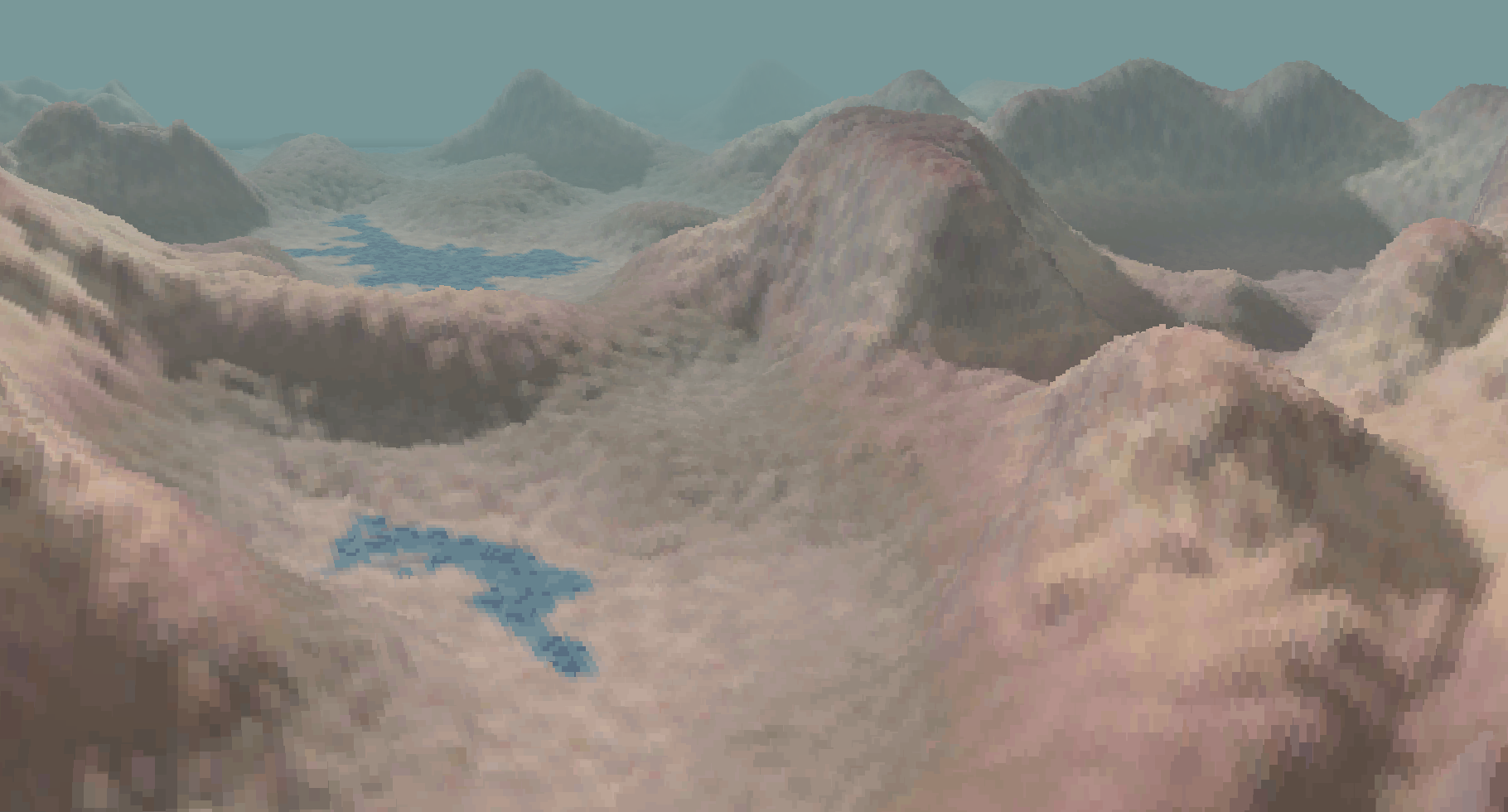
Bilinear Filtering
The game Outcast ( Appeal, 1999 ) made some changes to this algorithm, by applying linear filtering to the textures and using tiling resources instead of maps contained in a single image. It's hard to find much of anything about this game now, but this page has some information. In addition to the changes to the map representation, they kept depth information, and rendered polygons over the rendered result.
I tried filtering textures in my implementation, to see how it went - I'm not sure how much I like the look of it. It requires denser sampling of the textures, to avoid weird artifacts on the slopes between interpolated texels. You can see what that looked like, above.
Depth Fog
I thought this was implemented in an interesting way - by adjusting the opacity of the render target with depth, I was able to have the OpenGL clear color show through during the first pass. This was an easy way to create the colored fog, but it may be more efficient to disable depth testing ( as this main render texture is drawn with the use of a triangle, to blit to the screen surface ) and simply draw that first pass with a blended color, weighted by the same logic, and skip the API clear call altogether.
Since the operation to draw the computed minimap over the main rendered output is done as a second pass, the alpha blending for that pass will still work as intended. I'm not sure how much time it would actually save, but this may be a good change to make to the implementation.
Application: Visualizing Hydraulic Erosion Simulation
This draws from some code that I wrote a while ago, which was closely modeled after this implementation by Nicholas McDonald. It uses particles moving around a heightmap, picking up and depositing sediment, to model the natural process of hydraulic erosion. Much like the real phenomenon, this is a heavy process, requiring a large number of particles to be run before any significant changes in the terrain can be seen.
Initially, I tried running the whole program as a single threaded process, as before, but now with this update running between the rendering of frames. This caused a significant delay between frame updates, as a significant amount of work had to take place to compute the update and prepare the textures to send to the GPU to render. I spent a while thinking about how to fix this, and arrived at the current implementation. This creates a worker thread, at the beginning of the program execution, and has it a sequence of functions: run the simulation update with a configured number of simulation steps, then prepare the texture data as uint8 buffers which are ready to be sent directly to the GPU, and then set a completion flag. The main thread sees this flag, and resends the textures, invokes the shaders to compute the color data, and then presents it. If the flag indicates that the worker thread is still computing the updated data, the rendering process runs as it normally would, using the data that has been most recently been sent to the GPU.
This method, keeping this heavy work out of the main rendering thread, prevents any kind of hang between frames. The buffering of a 1024x1024 texture and running of the texture generation shader do not cause any perceivable hang. It all takes place well within the 16ms frame budget for 60fps, as the two render passes take a total of about 3ms.
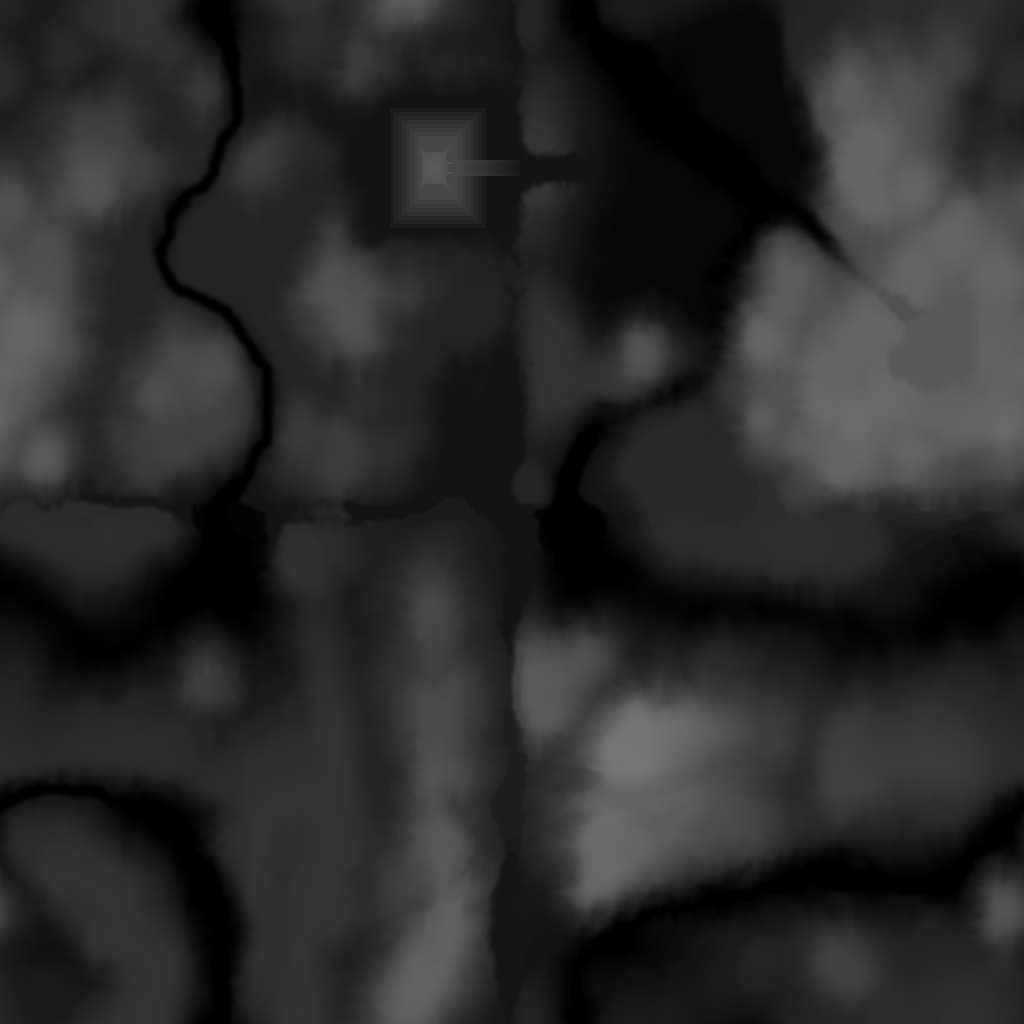
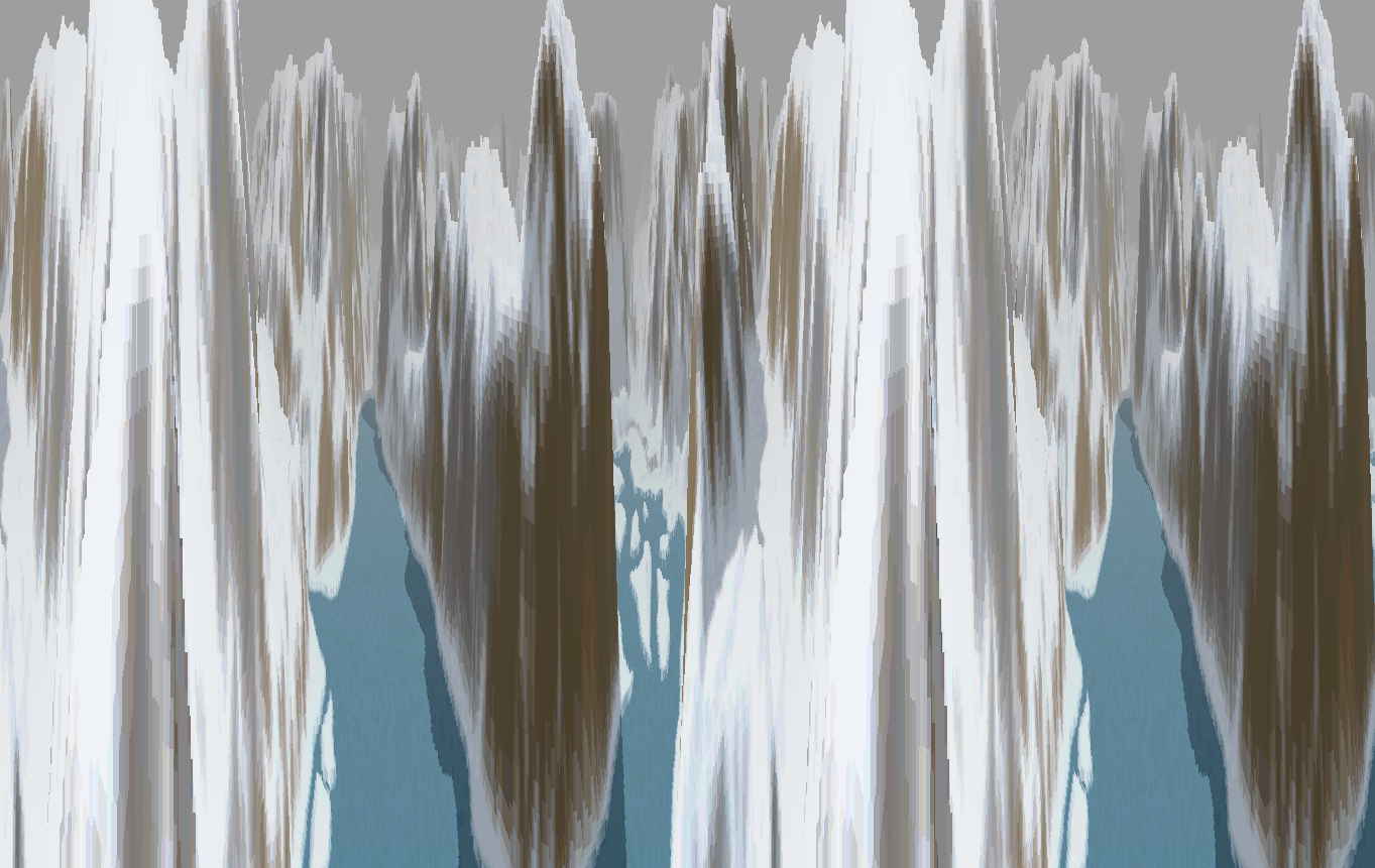
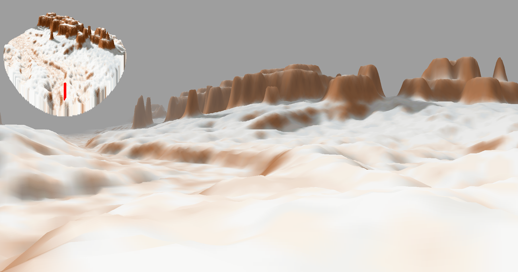
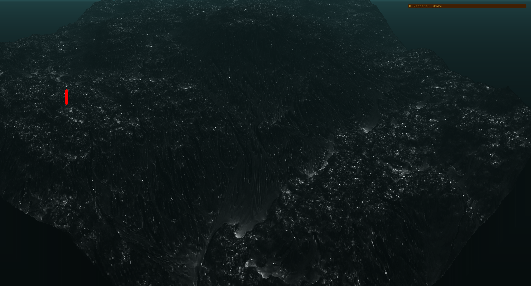
To generate the view you see above, there are a few contributing factors. The worker thread produces two textures, which are fed as input to the heightmap and colormap on the GPU. The heightmap contains the height data, but the colormap initially contains the normals, which are computed as part of the hydraulic erosion code, to inform the acceleration of the particles as they flow downhill. You can see what that input data looks like, here:
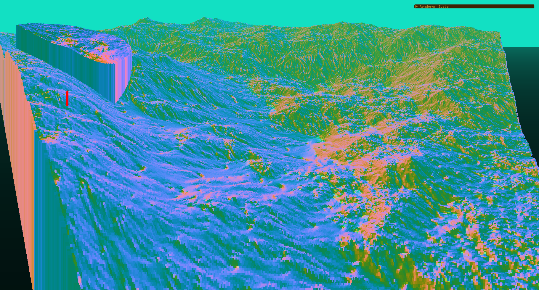
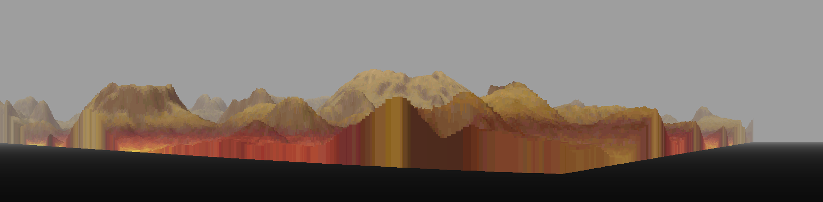
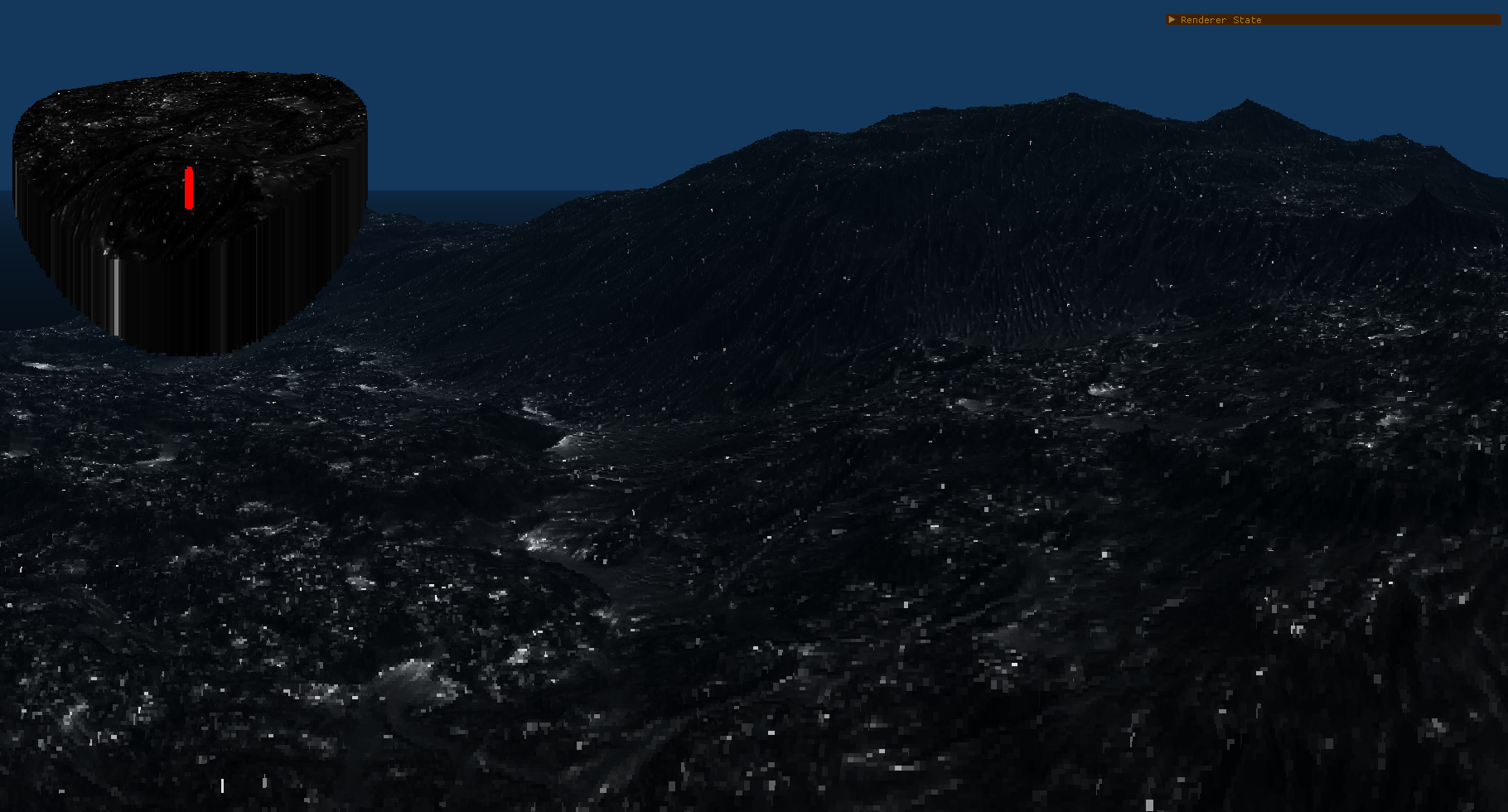
This data is used to compute diffuse lighting based on the dot product of the normal with a vector pointing straight up. This manifests as light colored highlights on flat surfaces, with steeper slopes getting progressively darker. You can see what this looks like, by itself, in these next two images:
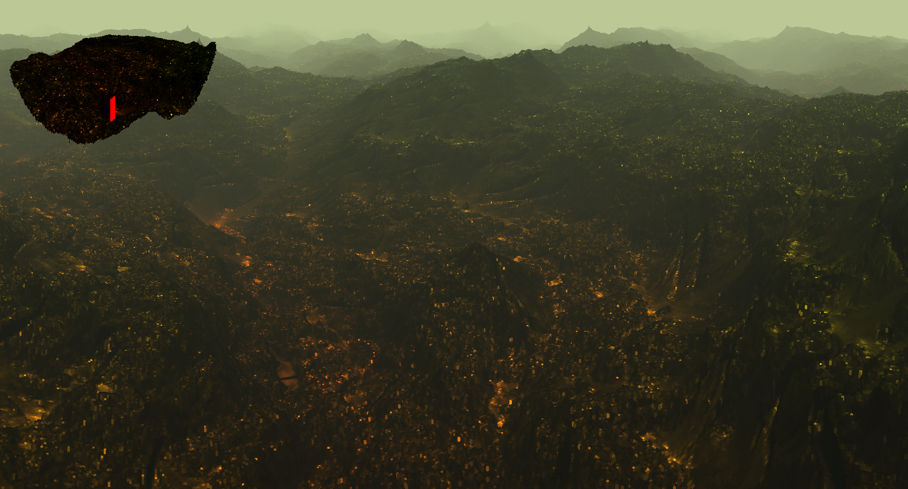
By multiplying a height based gradient from yellow to green by this diffuse lighting value, you can start to see some more interesting results like this:
Future Directions
As you can see in these couple images above, the computed output does not have shadows calculated upon the colormap. An interesting thing to add to the coloration shader would be traversal of the map, to check for occlusion, and adding some shadow contribution to the color output. There's a lot of headroom left, timewise, for this type of processing. In addition to this, I have a number of other ideas that may be directions worth pursuing. These might be exercises left to the interested reader:
- The efficiency improvements I mentioned earlier about disabling depth testing, blending color for depth fog rather than the hacky solution of using the alpha channel and the API clear color, perhaps using some different falloff curves, e.g. sigmoid
- Use of mipmapped texture sampling, manually adjusting LoD and step size as the renderer samples farther away from the viewer ( similar to the concept of cone tracing, brought down a dimension )
- Correcting the view distortion and curvature, by projecting the rotated direction vector onto the forwards vector and correcting length with respect to the view vector, to better replicate the sample position interpolation logic in the original implementation - it may be interesting to try the logic that was used in the original implementation directly, instead of the method I used with the rotated view ray
- Adding a soft edge falloff for the minimap texture at the edges of the masked circle, so that it fades out with reducing alpha, rather than the hard edge it has now
- Better shading, more interesting use of the shader's input data, as it is generated from the erosion sim
- Keeping a depth buffer and doing some other kind of rendering over this result ( polygons, sprites, raymarching ... ) or else postprocessing which could make use of this data
- Keeping a buffer of world X and Y, in the style of Vertexture and my chess implementation, which show X and Y encoded in the red and green channels, and using the information in this buffer to drive user interaction ( clicking would be able to pick values out of this buffer to immediately know world X and Y at the click location, perhaps for targeting, terrain manipulation, or placement of objects )