aiExperiments: Agent-Based Simulation with Simple Neural Networks
This was inspired by this implementation by Johan Eliasson. I was pretty fascinated by the process of these little neural network driven cars, which in effect had no idea what they were doing - this is due to the nature of neural networks - they have no explicit decision model, and instead construct some output values from some set of input values, filtered through some sets of hidden layers. I will explain.
Neural networks are actually a very elegant way to represent high order relationships between a set of inputs, when generating some output values. I referred to this set of tutorials, which explain the basics in simple terms, in a very transferrable way. This type of logic has a lot of different applications - I used it here for a very simple agent-based simulation, trying to create cars which could navigate their way around a track.
Neural Network Ultra-Basics
You hear the term neural network tossed around a lot these days, but never in a way which makes it very clear what exactly is taking place. A neural network is simply a feed-forward network of neurons ( for our purposes here, I believe there are implementations that use some stateful feedback ), a directed acyclic graph, which takes in some set of inputs to produce a set of outputs.
They are organized into layers - the input neurons, sense neurons as you might also call them, are the first layer, and feed into the first hidden layer. Here it makes sense to examine what exactly is happening inside of a neuron, as we now have a neuron with a set of inputs. These layers are 'fully connected', this means, that each of these neurons in the layer has connections to all neurons in the previous layer. This set of connections comes with a set of numerical weights, which express the role that they play in the generation of the output for the given neuron. When the neuron is evaluated, the activation values for each of these sense neurons are brought together into a weighted sum, and added to a per-neuron bias value. This weighted sum + bias is the output of the neuron, and is what is visible to the next layer of the network.
This process is recursively applied, until you have generated values for the output nodes. Sometimes, there are activation functions like sigmoid or RELU applied to the output values, to condition the values and prevent instability by constraining them to known ranges. For this application, I used the raw computed output of the offset weighted sum for all nodes, with no conditioning. The video below shows a couple runs of the simulation, with randomly generated weights and biases.
Implementation
Sprite Rendering
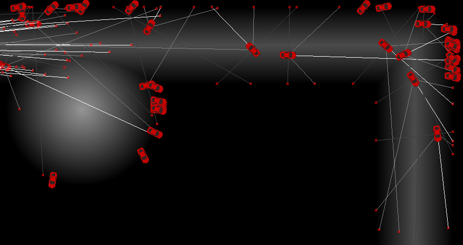
This was implemented as a simple layer over the SDL2 2D renderer, which allowed drawing of lines, rectangles, and oriented sprites. Each agent draws lines for the distance queries, best-guess intersection points for the edges of the road, and then an oriented car sprite to show its location. The agent's orientation, etc, is used to draw its representation as the simulation takes place across updates.
Track Representation & Reasoning
I selected a signed distance field based track representation for a few reasons. First, it can be laid out very simply - what you see here is four line segments and a circle. Second, it can be used by the simulation agents to get cheap and easy distance queries at different angles in front of them.
During startup, the SDF representation is queried at all texel locations on a SDL texture, which you can see in the grayscale representation in the video above - towards white is more negative, e.g. further inside the bounds. For this application, what I did is probably a bit overkil, but for more complex signed distance fields, this type of caching can greatly reduce the distance query time, by keeping precomputed distance reads for all points in the domain. Note that there will be some quantization artifacts, as texels are integer indexed - even with interpolation, there may be some artifacts which could cause trouble, depending on application.
Neural Network
This is the meat of this project - the inputs to the neural network are the distance queries, the speed, and the current orientation. I wrote it such that there could be an arbitrary number of layers, and an arbitrary number of neurons in each layer, but decided upon using two hidden layers of four neurons apiece. This then produced two output values, which were interpreted as speed adjust ( +/- ) and rotation adjust ( +/- ). Using a larger number of hidden layers maps to being able to represent higher order relationships, as there are more offset weighted sums computed in sequence, but it becomes more and more difficult to tune these relationships to be meaningful in any way.
With basically nothing more than the amount of knowledge I described above, I made some logic to compute these offset weigted sums. The values feed forwards from the input, to generate the output values, per simulation agent, per simulation update. There is just a std::vector of layers, which are each a std::vector of neurons. The input layer is populated from the distance queries and simulation agent parameters, then the first hidden layer is evaluated, then the second, then the output. The output values are then used to update the agent parameters going forwards.
Breeding and Evolution ( Read: Where a Roadblock Was Hit )
Typically, this is implemented using a method called backpropagation, by which a changes in a fitness metric are measured with respect to changes in the weights and biases. This gives you a model of derivatives with respect to these values, and gives you a way to tune your network weights and biases towards your fitness metric. Where this fell down was fitness metric - I initially thought to use the number of simulation updates which the agent survived for, before hitting a wall - as you can see in the video, there's a lot of degenerate cases, where the generated set of weights and biases make a simulation agent spin in one spot, never moving, or else go in tight circles.
To some extent, this could be mitigated with a system of checkpoints, or some other way to tell how far it has traveled along the track. Another approach might be to kill off agents that stayed within a certain distance of the starting point after some amount of time, but that wouldn't do that much. This may be something to return to in the future, but I was surprised by how well it worked, all things considered. As you can see, out of batches of about 200 simulation agents, between one and four have a network which is fit enough to make a full circuit of the track.
Something else that I think would be an interesting extension of this, is to consider extending it to three dimensions. I have thought about this before, but here it's come up again. By taking the distance queries at different points on a hemisphere in front of the agent, this may be a relatively trivial extension to the existing logic. I saw this today, which seems like an interesting environment for this simulation to take place in. Might also be interesting to do it in compute, to handle a large number of them at once.