Adam: An Interesting Interlacing Scheme
What is this? Good question. It's kind of an interlacing scheme, kind of an interpolation scheme, kind of a shitty denoiser for sparse point samples. It's loosely based on the adam7 interlacing algorithm. Where adam7 operates in 8x8 blocks, the algorithm presented here generalizes to any power of two square texture (and nonsquare, by rounding up to the next power of two) using the mip levels of the texture.
Background
The application, here, was based on my fascination with the progressively increasing resolution of this renderer on shadertoy. You can see that it starts with a very blocky version, with large pixels, refining into higher and higher resolution until it has per-pixel detail. I think this is very interesting to watch as it runs. I have been thinking about this on and off for a couple months, how you would approach this problem, how you could do it in a way that varied the level of refinement across the image.

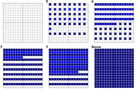
Adam7 is a little bit strange, because it does the axis splits separately. By this, I mean that the first level of refinement has only one pixel in the block. You can imagine that this pixel now is duplicated for every pixel in the block, we have one piece of data. The second level of refinement adds another pixel in the block... and you can visualize now with a split on the X axis. That is, now, for each 8x8 block you can visualize the data as 2 separate 4x8 blocks - one for each filled-in pixel - to cover the entire footprint of the block. The third level, you're now doing a split on the Y axis, filling in two more pixels. Once it completes this third level, you can visualize it as 4 separate 4x4 blocks. It follows this pattern you can see here until all pixels have been filled in, and the blocks become 1x1, full resolution.
I did this out on paper, and figured out the progression, how to do the floor logic so that each pixel references the nearest filled in pixel... but getting into the implementation, there's a bit of a hitch. If you want to try to use the levels of a texture to represent it, you run out pretty quickly. This is because the purpose of texture levels in the OpenGL API is for mipmapping, that is, hierarchical pre-filtered versions of the first level of the texture, halving resolution on both the X and Y axes at each level. The specifics are out of scope, but the general purpose of a mipmap is to both improve performance by reducing required texture bandwidth when sampling, while at the same time also helping reduce aliasing when sampling a texture mapped onto a distant object.
The point is - the API design is such that you are only given enough levels to create a complete mipchain for the largest texture that the API can create. Most modern systems that I've seen, the value of GL_MAX_TEXTURE_SIZE is 16384. This is 214. The "typical" maximum number of levels, which comes as a consequence of this... is log2(GL_MAX_TEXTURE_SIZE), because a maximum sized texture will need that number of levels to get down to a single texel in the highest mip level. For this resolution, we get log2(214) = 14 levels.
Well, if you want to split on each axis alternately in the style of adam7, you'd be using two levels for each level in the mipchain style approach. Without adding a second texture, and the added complexity that would come with that... you can only support 27 levels of refinment, meaning a maximum resolution of 128x128 pixels. That's significantly lower than I wanted - my intention was to be able to use this in a similar manner as the shadertoy example above, as a render preview. I want to be able to do resolutions at least up to 4K, and maybe crazy triple monitor desktop background resolutions like 7560x1440 pixels.
Long story short - I ended up just using a mipchain, and doing the axis splits together. This makes a structure sort of like a quadtree, just like a regular mipchain, where each texel in mip N+1 represents an averaging of 4 texels in mip N. This is better in a couple ways... reduced memory footprint relative to the doubled levels, and much less complexity for the offset calculation logic (it just becomes factors of two).
How it Works
The operation works in two pieces. First, you need to generate the mipchain - this is very similar to standard mipchain generation, with some small changes. Second, you need to step through levels of the mipchain until you find the lowest mip level that has data. Mip 0 is full resolution, mip 1 is half on each axis... down to a single texel in mip N. An interesting consequence of this is that data will propagate all the way up the mipchain, and fill in gaps in an incomplete image (more on that in a bit).
Generating
There's two relevant pieces of data. Designing for my usecase, a renderer which stochastically fills in pixels across the image... I'm keeping four channels - a three-channel color value and what is essentially a bool "is there data for this pixel in mip 0" in the alpha channel. I write 1's in mip 0, but it will use a range of alpha values to represent the sum of contributing pixels as it progresses up the mipchain. For convenience, we'll call these values "color" and "count".
The mipchain representation here is calculated by doing a sort of masked/weighted average over the filled in pixels. When data is added to mip 0, a color is set, and a 1 is put into the alpha channel to indicate, "we have data here". Calculating mip 1, we consider the four contributing texels in mip 0. We get a weighted average, multiplying the color values by the count values (either zero or one), and normalizing by the sum of the counts. The value that is written to mip 1 is the normalized average color, and the sum of the count values in the alpha channel. The reason for maintaining this count value is so that we are only averaging pixels that contain valid data.
As you progress up the mipchain, you are getting averaged colors, and total counts for each texel. I'm keeping full-fat 32-bit floats, because my use case will need to pull out that data for EXRs. With that pretty heavy data footprint, the total computation time for this mipchain is about 0.7ms on my Radeon VII machine. You can find a reference implementation of the shader used for this generation step, here. Invocation is handed exactly the same as standard mipchain generation.
Sampling
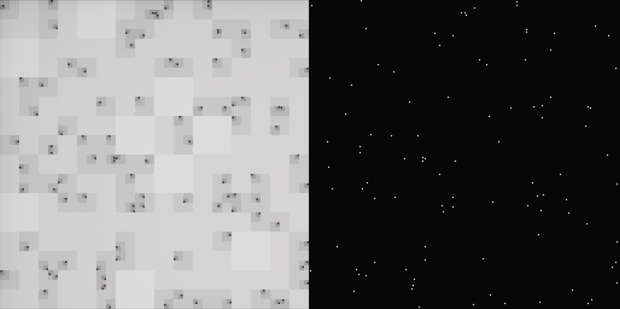
Now that the mipchain has been populated, sampling each pixel on the image is an iterative process to find the lowest mip level that has data. You might have noticed, a consequence of the weighted averaging... as long as a single pixel in the image is filled in, mip N will have something in it. Starting at mip 0, and going up to mip N, you stop at the first mip level you encounter with a nonzero count value, and take the corresponding color value for the output. Having to go to higher mip levels maps to bigger blocks. You can see a simple visualization here, with only a few point samples filled in. On the right, mip 0, on the left, pixels get brighter as they go to higher mips. Mip 0 is black, to white at mip N.

I'd like to eventually try visualizing this as a heightmap or stack of planes, masked to the regions that are filled in. Areas that have per-pixel detail in mip 0 would be at the top, and the solid color single texel at mip N would be at the bottom.
Filling in Gaps
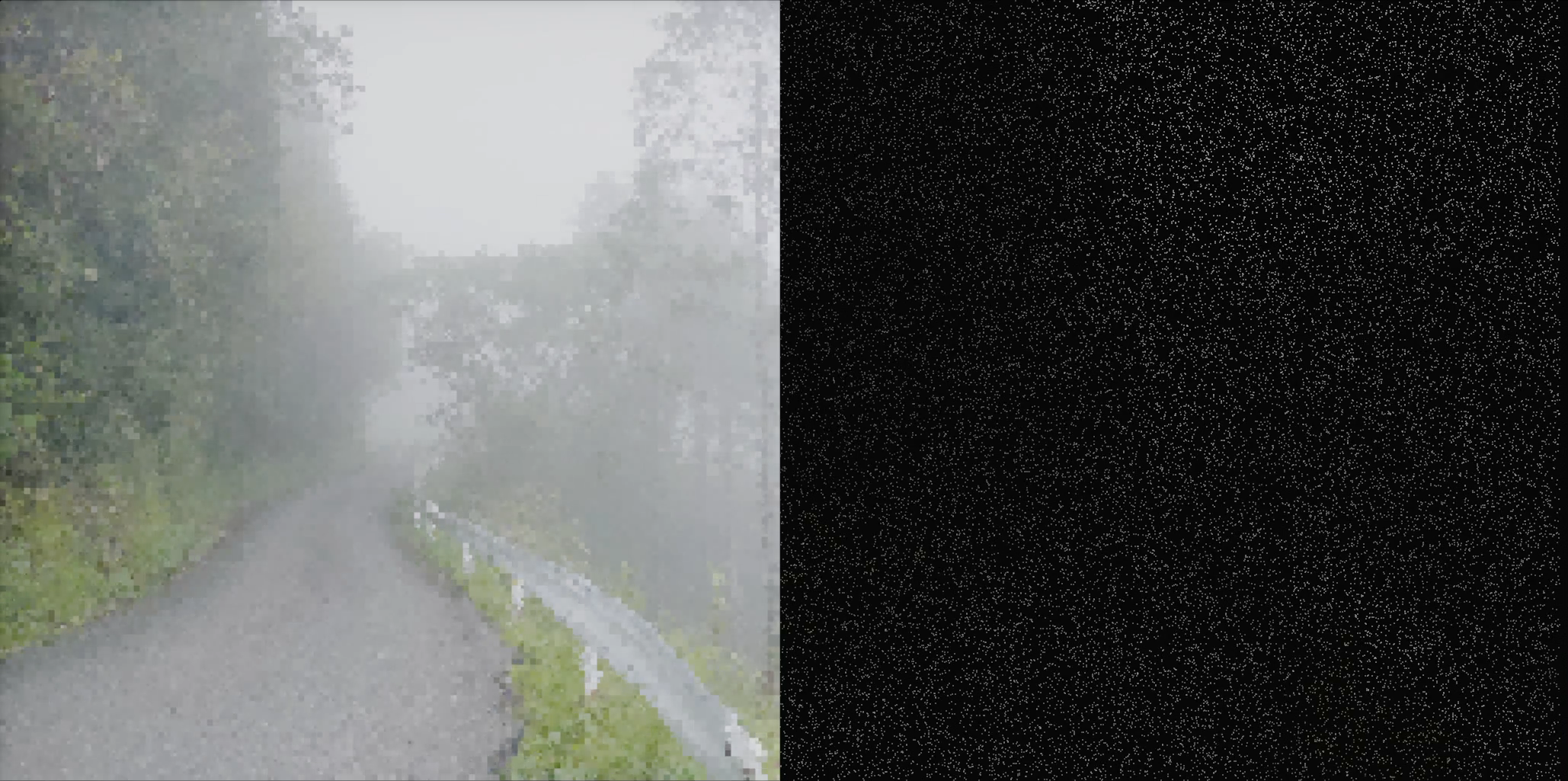
I mentioned how this could be understood as a shitty denoiser, filling in gaps in sparse point sampled image data. What I think is really interesting is that if you have a single mip 0 texel filled in, it will propagate up to mip N. And because there's no other pixels contributing to the weighted sum at any stage, the entire image will be filled with the exact color of that single texel. There's interesting implications here, for filling in gaps in an image. What you can see here, is an image with a little more than 97% of the pixels removed. It looks like less because of linear filtering, but the point is - on the right you can see the contents of the "color" component of mip 0, and on the left you can see the image sampled from the representation described here.

I think this is really interesting, because the point samples don't even look like anything. It's very lossy, but you do get something that plays much nicer with your sense of sight, and creates a visually pretty complete image. I was surprised by just how much this subjectively improved things from such a small amount of remaining image data.
Future Directions
I've been enjoying mythological names for my projects lately. Interesting implications as it relates to christian mythology, one propagating to many... In any event, the intended usage here is as part of the interactive viewer component of the next pathtracer I'm working on, Icarus. The idea there is that it is a wavefront pathtracer, and will be doing some interesting stuff to run a lot of samples for a small set of pixels each frame. More on specifics, upcoming. The point is, this matches this behavior that I'm showing in the videos above... filling in some set of pixels stochastically, each frame. I'm glad that the computation and sampling of this representation does not create a lot of overhead, it will be a nice fit for this renderer.

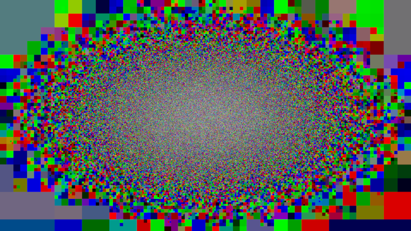
Another thing that I think is very interesting is how you can use this for foveated rendering. Designing for this renderer and the intended behavior as a preview that fills in quickly, you might want more detail towards the center of the image, maybe that's the focus point of your rendered view. By filling in mip 0 pixels based on a gaussian distribution, centered at the middle of the image, you get more detail in those texels near the center of the image. You can see how in the periphery the detail falls off, having to reference higher and higher mip levels before getting usable data.
A couple people have shared some related research topics, that I will share here for anyone that is interested: