This project focused on developing some new techniques based on some more interesting features of OpenGL 4. OpenGL 4.1 introduced compute shaders, and OpenGL 4.2 introduced Image Load/Store functionality. Where a 3D texture is read only in the shader, I found out that the corresponding Image3D objects provide a load/store interface that allows for arbitrary reads and writes from your shader programs. The value in this, to me, was the ability to use these large chunks of texture memory to compute cellular automata on large 3d grids, additionally using the parallel nature of the GPU to assist in making this a realtime venture.
Though this project implements the same new voxel raycast rendering scheme that is present in Voraldo 1.0, I am going to go into more detail in the writeup for that project and here focus more on what makes this project different from 1.0. The video is a little jumpy because the CA updates are done manually with a keypress.
This started with a curiosity about textures and the kinds of things that are possible to do with them – one of my first thoughts was, ‘do you have write access?’. Turns out, no, you do not have write access with standard textures. I was not convinced that this was a hard limitation based on some things I had seen done, and through some research and asking around (huge thanks to Eric Arnebäck, who helped me a lot in figuring out how the initialization and use differed from standard textures), I found out about Image Load/Store which was intended to serve this purpose. This set of functionality gives you image objects in GLSL – this is different from a sampler, which takes normalized coordinates (coordinates fall in the floating point range 0-1) and is read only, in that all references are done with ivecs (integer vectors, which refer to specific pixel/texel offsets), and you have functions to both load info from them, and store info to them.
CELLULAR AUTOMATA
This is a deeply interesting concept that I came into contact with early on in my Computer Science career – I believe the first one I encountered was Conway’s game of life, I thought the organic nature of the patterns and the logic of ‘my next state relies upon my current state and the current state of my neighborhood’ was incredibly fascinating.
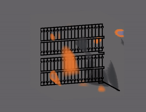
There are many different implemented algorithms, representing a number of things including fire, water and sand-type powders – the one I picked for this project is a classic 4-state automata called WireWorld, which takes a very simplified/discretized view of the flow of electricity through a wire. There are 4 states - conductor, electron head, electron tail, and empty (this contains anything that’s not the exact colors associated with the other three states). It was initially conceived as a 2 dimensional cellular automata, but the logic generalizes perfectly to 3 dimensions. There are no changes in the rules – they are simple – two unconditional ones – electron head becomes electron tail, electron tail becomes conductor. Another, sort of trivial, empty is unaffected and just gets written with it’s previous value. Slightly more complicated is the behavior that’s core to what makes wireworld’s behavior so interesting (check out my 2d example on the javascript/canvas demos page) – basically you’re looking at the neighborhood of any cell that’s in the conductor state - if either one or two of the cells in the neighborhood are in the electron head state, you will become the electron head state. If there is greater or less than that amount, you remain a conductor.
This simple set of rules establishes a system in which you can create diodes, logic gates, building up to complex digital circuits if you want. I find this as an example of a cellular automaton incredibly fascinating. Game of Life is neat, but the behavior of WireWorld is something that can be much more easily engineered into functional units (in my mind anyways, I’m very comfortable with digital logic systems based on boolean values from my EE/CS stuff in school) – I’ve seen this extended in 2d into small scale digital computers with ROMs containing instructions that it’s able to read and use. I like the idea of this modeling the electrical system on a vehicle, combined with a voxel based damage model you would have the basis of a very interesting little structure.
COMPUTE SHADERS
That’s all well and good – but how is it implemented? The most obvious choice is OpenGL 4.1 Compute Shaders, which are parallel programs on the GPU, independent of the standard rendering pipeline, and allow arbitrary operations on buffers you set up on the GPU. The way these jobs are dispatched allows for each invocation to have a unique 3 dimensional ivec address kept in gl_GlobalInvocationID.xyz. This maps perfectly to the structure of the image load/store objects. This is the method I have taken in Voraldo 1.0, and it’s a much smoother way to do it – the method used for my final project did not use compute shaders, but instead modeled this behavior using a concept called attributeless rendering. Based on time constraints for the final project, I didn’t have time to find example code for a compute shader to get that rolling for this one. I didn’t realize how simple it was to set up yet, so I had to do a bit of a workaround.
In this attributeless rendering schema, you compile your ‘pseudo-compute’ shader just like you would any other set of vertex and fragment shaders – you leave your fragment shader effectively empty, since it will be doing no work. A key element is that it does not use any attributes – that is, there is no per-invocation data that is passed in, such as verticies, colors, normals, texcoords, etc. Instead, I calculate an X, Y and a Z from gl_VertexID, which is a built-in variable that identifies which invocation of the shader you are dealing with. By calling glDrawArrays with the number X*Y*Z, you get X*Y*Z invocations of the shader and gl_VertexID ranges from 0 to (X*Y*Z)-1.
It’s a simple operation to do a little bit of mod logic to get the equivalent to gl_GlobalInvocationID – once you have that, you can reference the image for the previous state and neighborhood, then compute and store your new state at that same address.
SYNCHRONIZATION
So far, I’ve avoided any discussion on how this is synchronized. There’s an issue in that the ~33 million invocations of the pseudo-compute shader are not truly parallel, in the sense that they execute purely at the same time, with the same initial conditions. If you were to model this with a single Image3D object, you’d have a strong likelyhood of ‘stepping on your own toes’ - that is, polluting the image3D and injecting some order-dependence into something that should be pretty trivially parallelizable.
Simple fix – keep two image3Ds, and ping-pong between them each frame – one represents your 'current' state, one represents your 'previous' state. Each frame, you’ll be reading from your 'previous' state, writing to your 'current' state, then swapping buffers, so that the 'current' becomes the 'previous', and the 'previous' becomes invalid data that can (and must be) written over, as the next 'current'. If you don’t write to it, you’ll have data stored that’s propagated from more than 1 frame ago, which is not what you want here.